Signed Distance Functions Techniques
A Signed Distance Function provides a way to describe geometric forms in a continuous manner by associating each point in space with its signed distance to a surface.
The function returns a positive value when the point is outside the shape and a negative value when inside. This framework is highly flexible, allowing the representation of shapes in 2D, 3D, and even N-dimensional spaces, since the Euclidean distance is not restricted to a particular number of dimensions.
A defining feature of Ray Marching is its use of signed distance functions to describe geometry, rather than traditional vertices, edges, and faces. This approach is precisely what makes Ray Marching a powerful technique, capable of rendering smooth surfaces, shapes distorted by procedural noise, repetitive patterns, and dynamic shapes that evolve over time.
Basic Shapes
The general form of an SDF function includes:
- $\mathbf{p}$, the query point, for which the distance from the shape positioned at the origin is computed.
- Shape-specific parameters, such as the radius for circles and spheres, or additional properties like width, height, or orientation for more complex geometries.
Circles and Spheres
For a circle centered at the origin in $\mathbb{R}^2$ with radius $r$, the SDF is:
$$\text{CircleSDF}(\mathbf{p}) = \|\mathbf{p}\| - r$$
A sphere in three-dimensional space follows the same principle. If the sphere is centered at the origin with radius $r$:
$$\text{SphereSDF}(\mathbf{p}) = \|\mathbf{p}\| - r$$
The only difference is the dimension of the query point $\mathbf{p}$. In the case of a circle, $\mathbf{p}$ is a two-dimensional vector; for a sphere, $\mathbf{p}$ is a three-dimensional vector. The formula is structurally identical because both objects are defined by a center and a radius in their respective spaces.
float circleDistance(vec2 point, float radius){
    return length(point) - radius;
}

float sphereDistance(vec3 point, float radius){
    return length(point) - radius;
}
Code 2: Circle and Sphere SDFs
Since an SDF returns a positive distance when a point is outside the primitive and a negative distance when inside, this information can be used to assign different colors to a 2D shape rendered on the canvas.
vec3 plainColor (in float d){
     return vec3(1.0) - sign(d)*vec3(0.4);
}

void mainImage( out vec4 fragColor, in vec2 fragCoord )
{
    vec2 uv = (2.*fragCoord.xy-iResolution.xy)/min(iResolution.x, iResolution.y);

    float d = circleDistance(uv, 0.5);

    vec3 col = plainColor(d);
    fragColor = vec4(col,1.0);
}
Code 3: Rendering Circles

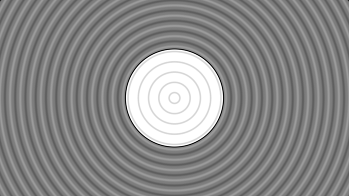
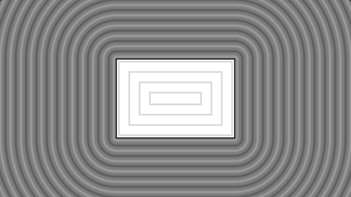
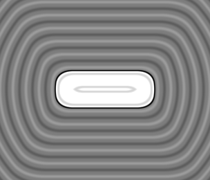
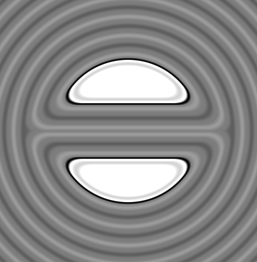
In Figure 7, the color outside the circle is rendered in a darker shade than inside. For the following shapes, a custom coloring function adds isolines and highlights the border, as shown in Figure 8. This technique allows the visualization of 2D SDFs in the distance space.
3D SDFs define the shapes of objects within a scene in the Ray Marching pipeline. The following examples illustrate 3D SDFs rendered with Lambertian diffuse shading and Phong specular reflection. Since lighting models are outside the scope of this work, readers may refer to [Akenine-Möller, 2018] for further details.
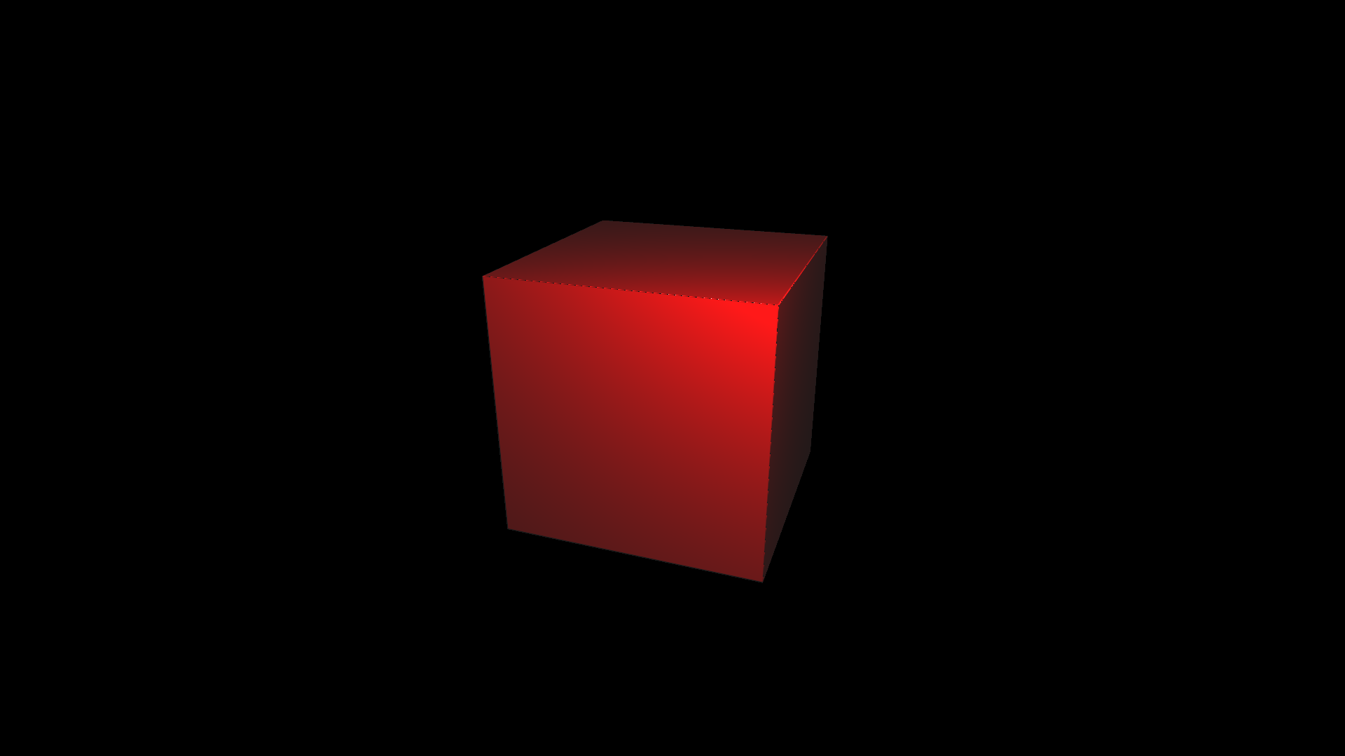
Rectangles and Boxes
Similar to the 2D circle, the SDF of a 2D box (rectangle) can be generalized to higher dimensions.
float rectangleDistance( in vec2 p, in vec2 b ){
    vec2 d = abs(p)-b;
    return length(max(d,0.0)) + min(max(d.x,d.y),0.0);
}

float boxDistance( in vec3 p, in vec3 b ){
    vec3 d = abs(p)-b;
    return length(max(d,0.0)) + min(max(d.x,d.y,d.z),0.0);
}
Code 4: Rectangle and Box SDF
The rectangle SDF is defined at the origin $(0,0)$. Due to the rectangle's symmetry, it is convenient to work within the first Cartesian quadrant. $\mathbf{b}$ (half each box's side) is subtracted from $\text{abs}(\mathbf{p})$, yielding a point $\mathbf{d}$. As illustrated in Figure 11:
- If only $\mathbf{d}.x < 0$, $\mathbf{p}$ is above the rectangle — the shortest distance is straight down.
- If only $\mathbf{d}.y < 0$, $\mathbf{p}$ is next to the rectangle — the shortest distance is straight left.
- If both $\mathbf{d}.x < 0$ and $\mathbf{d}.y < 0$, the point is inside — the shortest distance is the closest of the two sides.
- If neither component is negative, the point lies diagonally outside — the distance to the corner is the shortest.
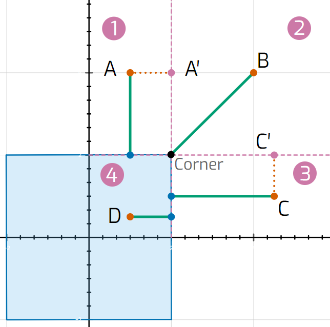
When both $\mathbf{d}.x$ and $\mathbf{d}.y$ are clamped to zero, length(max(d, 0.0)) gives the corner distance for all outer sections. For the interior (where that expression is always 0), the SDF must return the negative distance to the nearest edge via min(max(d.x, d.y), 0.0). This generalizes directly to $\mathbb{R}^3$ for the box SDF.
If expanded to $\mathbb{R}^4$, the SDF can help visualize forms such as the tesseract (the 4D hypercube) by fixing and scrolling through one of the four axes.
Basic Transformations
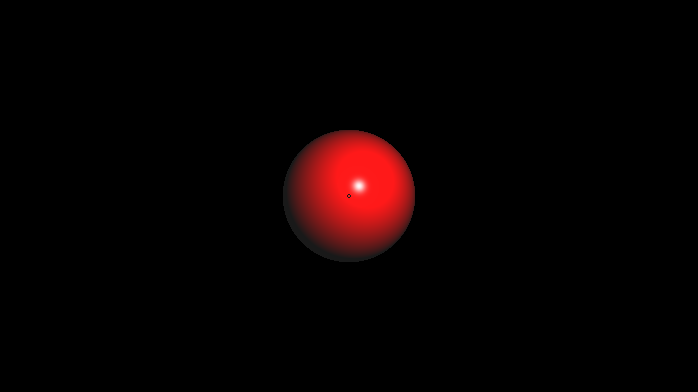
All primitives described above are centered at the origin. To perform a transformation such as scaling, rotation, or translation, it is possible to apply the inverse transformation at the query point $\mathbf{p}$ — transforming space rather than the shape directly.
In Code 5, by subtracting the vector $(0, 3, 0)$, the sphere is effectively positioned at $(0, 3, 0)$.
float transformedSphere(vec3 point)
{
    return sphereDistance(point - vec3(0., 3., 0.));
}
Code 5: Translating a Sphere
Affine transformations can also be composed using matrices. GLSL provides built-in support for creating and inverting matrices. Code 6 shows how different affine transformations can be composed.
float transformedSphere(vec3 point)
{
    // Scale 2X along Y
    mat4 S = mat4(
        vec4(1., 0., 0., 0.),
        vec4(0., 2., 0., 0.),
        vec4(0., 0., 1., 0.),
        vec4(0., 0., 0., 1.)
    );
    // Rotation in XY
    float t = PI/4.;
    mat4 R = mat4(
        vec4(cos(t), sin(t), 0., 0.),
        vec4(-sin(t), cos(t), 0., 0.),
        vec4(0., 0., 1., 0.),
        vec4(0., 0., 0., 1.)
    );
    // Translate to (-2., -1., -1.)
    mat4 T = mat4(
        vec4(1., 0., 0., -2.),
        vec4(0., 1., 0., -1.),
        vec4(0., 0., 1., -1.),
        vec4(0., 0., 0., 1.)
    );

    mat4 transformationMatrix = S * R * T;
    vec3 transformedPoint = (vec4(point, 1.) * inverse(transformationMatrix)).xyz;

    return sphereDistance(transformedPoint);
}
Code 6: Affine Transformations on a Sphere
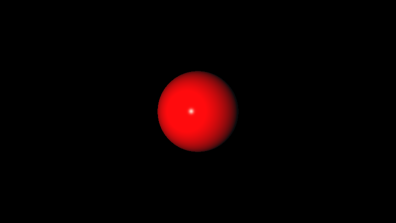

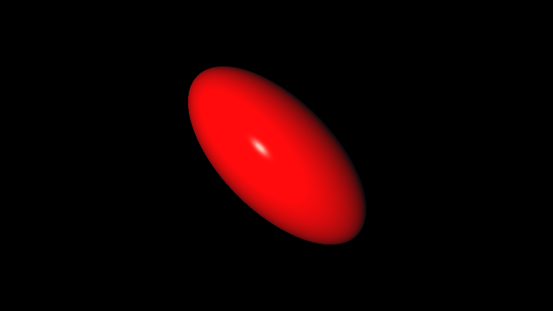
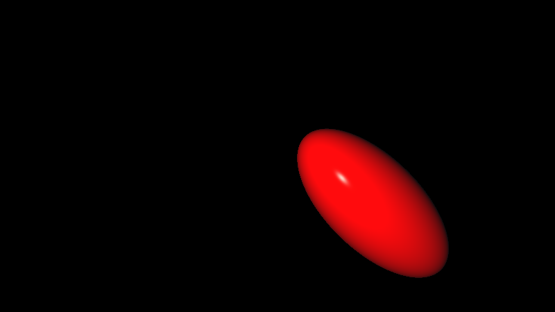
Figure 13 — Composing Different Affine Transformations on a Sphere.
Operations
While being able to display a variety of primitives is useful, building more complex forms is where Ray Tracing and Ray Marching part ways. While Ray Tracing depends on high polygon-count models, Ray Marching finds more success with combinations of primitives and operations as building blocks.
Union, Intersection and Subtraction
The most basic SDF operations are the boolean combinations: Union, Intersection, and Subtraction. These are some of the most elegant features of SDFs, taking as input the resulting distances of two primitive SDFs.
float unionOperation( float d1, float d2 )
{
    return min(d1,d2);
}
float intersectionOperation( float d1, float d2 )
{
    return max(d1,d2);
}
float subtractionOperation( float d1, float d2 )
{
    return max(-d1,d2);
}
Code 7: SDF Union, Intersection, and Subtraction
From the perspective of a 3D raymarched view:
- Taking the minimum between $\mathbf{d_1}$ and $\mathbf{d_2}$ renders only the closest surface from both objects — the union.
- Taking the maximum means nothing outside the intersection of both objects is visible, since the ray march only considers a hit if both SDF results are below the hit threshold.
- Taking the maximum between $\mathbf{-d_1}$ and $\mathbf{d_2}$ intersects with the inverse of object 1, resulting in the subtraction of object 1 from object 2.
Figure 14 illustrates these constructive solid geometry operations between a cube and a sphere.
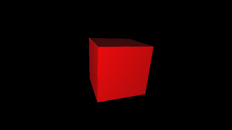
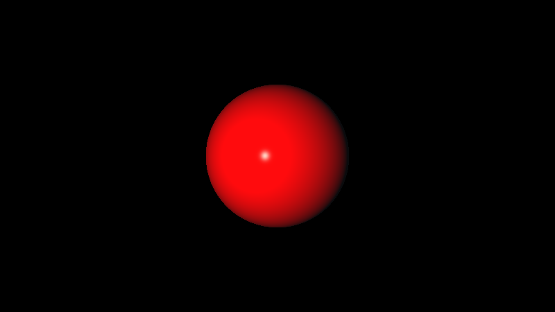
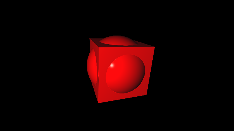
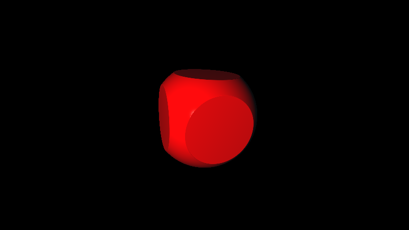
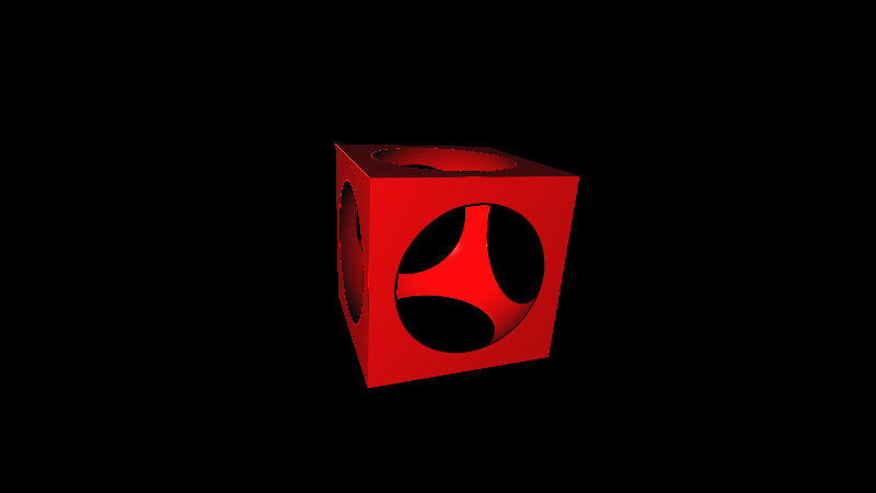
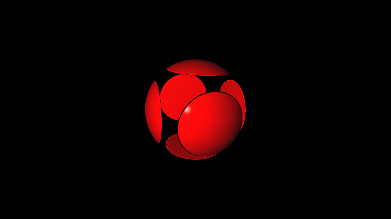
Figure 14 — Raymarched Constructive Solid Geometry Operations with Cube and Sphere SDFs.
Smooth Union, Intersection and Subtraction
A more visually appealing way to display boolean operations is through smooth minimum and maximum. Instead of hard edge transitions, it offers a smooth blend. This blending can be achieved through multiple types of functions — quadratic, cubic, exponential, sigmoid — each having its pros and cons [Quilez, 2013].
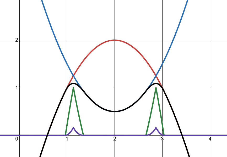
Because it is fast and does not overestimate distances, the quadratic polynomial is less prone to visual artifacts and is the most widely used version for Ray Marching. Similarly to the regular min function, smin (Smooth Minimum) takes inputs $\mathbf{a}$, $\mathbf{b}$, and the threshold $k$ — blending starts where the distance between $\mathbf{a}$ and $\mathbf{b}$ is smaller than $k$.
All polynomial methods start by finding the $h()$ function, which ramps from 0 to 1 as $|\mathbf{a} - \mathbf{b}|$ goes from $k$ down to 0:
$$h = \frac{\max(k - \|\mathbf{a} - \mathbf{b}\|,\; 0.0)}{k}$$
Next, a correction term $c$ is applied such that $\min(\mathbf{a},\mathbf{b}) - c$ produces the smoothed curve. For the quadratic version ($n = 2$):
$$c = \frac{h^n \cdot k}{2n}$$
Squaring $h$ makes $c$ ease into its peak rather than following a straight ramp. Multiplying by $k$ compensates for variation as $k$ increases. For smooth maximum, $\max(\mathbf{a},\mathbf{b}) + c$ suffices.
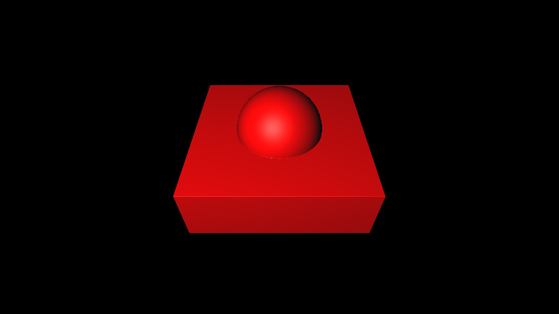
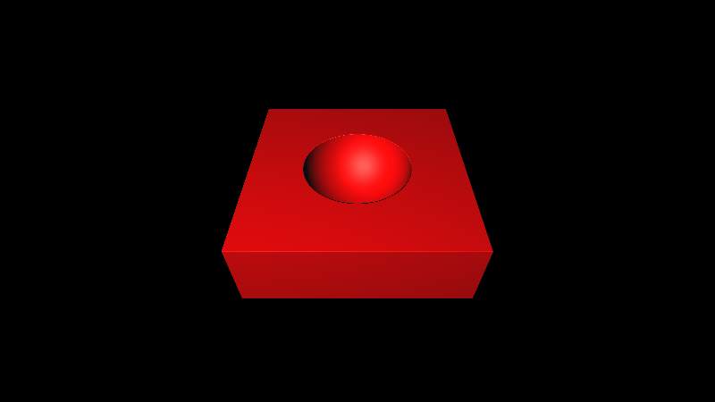
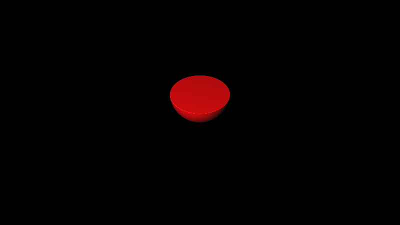
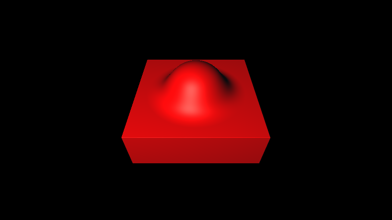
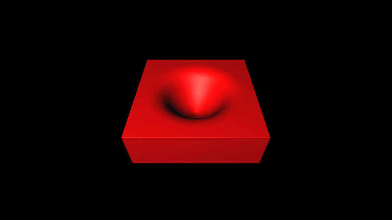
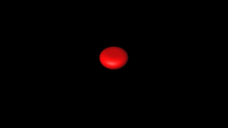
Figure 19 — Raymarched Smooth Operations with Cube and Sphere SDFs.
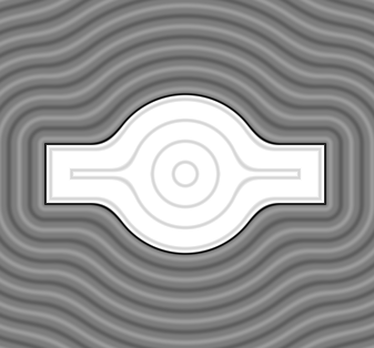
Domain Repetition
Since SDFs are expressed as mathematical functions, they can be transformed to repeat periodically across space. This technique, known as Domain Repetition, allows for the creation of infinite, repeating patterns while also optimizing performance by avoiding the need for multiple individual primitives.
Trigonometric functions such as sin and cos create natural repetitive patterns,
however bending the domain with these functions compromises the accurate
Euclidean distances the SDF relies on, potentially generating undesired
features. Functions such as round(x) or mod(x) are
more commonly used instead.
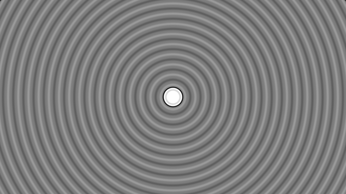
circleDistance(uv, 0.1)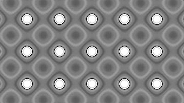
circleDistance(sin(uv*5.)*0.2, 0.1)
circleDistance(uv - round(uv), 0.1)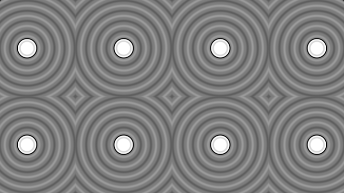
circleDistance(mod(uv, 1.) - 0.5, 0.1)Figure 20 — Examples of Domain Repetition techniques.
This can also be used in 3D. Given that $\mathbf{p}$ represents the query point, the repeated domain can be expressed as , where gap is the size of the repeated domain box.
sphereDistance(p - 6.5*round(p/6.5), 1.0) — infinite spheres from a single SDF.Displacement
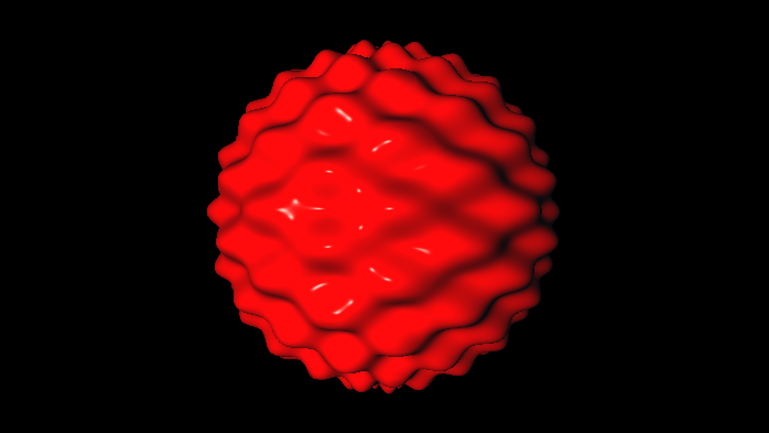
Displacement adjusts the geometry to simulate bumps or irregularities, adding fine detail to the surface. This is done by perturbing the distance field using patterns that look random, such as procedural noise or noise textures.
float displacementOperation( in sdf3d sdfShape, in vec3 p )
{
    float d1 = sdfShape(p);
    float d2 = displacement(p);
    return d1+d2;
}
Code 8: SDF Displacement
Although noisy functions are commonly used for displacement, any function can be applied to distort the distance field — enabling non-Euclidean effects such as bending or twisting space. However, this comes with a caveat: the sum of an SDF and an arbitrary function is not necessarily a valid SDF.
A key property of SDFs is that their gradient has length $1$ everywhere in space. When two SDFs are added, this property is violated — the gradient no longer has unit length, effectively "bending" space. This can cause the raymarcher to underestimate or overestimate the true distance to a surface. This issue can be attenuated by reducing the step size, though at a performance cost. In practice, small deviations rarely produce noticeable artifacts, making displacement through function addition still useful for subtle surface detail.
float distortedSphereDistance(vec3 p){
    float sphereRadius = 2.0;
    vec3 sphereCenter = vec3(0., 2., -5.);
    float sphereDist = length(p - sphereCenter) - sphereRadius;

    vec2 uv = sphereUV(point, sphereCenter); // spherical coordinate angles
    float distortion = sin(uv.x * 64.) * cos(uv.y * 64.); // wave pattern
    sphereDist += distortion * 0.1; // apply displacement

    return sphereDist;
}
Code 9: Wave Distortion on Sphere