Clouds
One of the main applications of Ray Marching is in the rendering of realistic smoke and clouds — volumetric objects that are inherently continuous and difficult to model with traditional geometry.
Clouds are mostly made of two main high-albedo types of particles (not considering dirt or other minimal particles): air and water/ice. Since clouds are not solid, when light hits them some rays bounce while some pass through the object. Furthermore, water particles are anisotropic, meaning that light tends to bounce differently depending on the direction from which it hits the cloud. All of this requires significant adaptation from the original Ray Marching approach.
Volumetric Rendering
To render gaseous materials, instead of avoiding surfaces, Ray Marching must
traverse into them. The SDF now represents density instead of
"distance to surface". The function is renamed GetDensity(p) and
follows these rules:
- If $\mathbf{p}$ is outside the primitive: yields a negative density (no density).
- If $\mathbf{p}$ is inside the primitive: yields a positive density, and the further $\mathbf{p}$ is from the bounds, the higher the density.
To consistently sample the density along the cloud, a constant step size is better suited. Instead of querying the scene's distance for the next step, each iteration advances by a fixed amount. This comes at the expense of performance, losing the sphere-tracing optimizations discussed in Chapter 2.
To mitigate the performance loss, an outer bound is applied to clouds. With a separate SDF, the bound acts as a regular surface — when hit, Ray Marching switches into the fixed-step mode.
PROCEDURE MarchRay(Ray, Scene)
  MarchDistance ← 0
  marchPos ← Ray.origin
  Hit ← NULL_HIT
  accColor ← (0, 0, 0, 0)   // RGBA: rgb = accumulated color, a = accumulated density

  FOR step = 0 TO MAX_MARCH_STEPS - 1
    marchPos ← Ray.origin + (MarchDistance × Ray.direction)
    Hit ← GetDist(marchPos, Scene)
    MarchDistance ← MarchDistance + Hit.distance

    // Hard surface hit
    IF Hit.distance < SURFACE_DIST AND Hit.material ≠ CLOUD
      accColor ← accColor + hitColor × (1 - accColor.a)
    END IF

    // Cloud bound hit: switch to fixed-step mode
    IF Hit.distance < SURFACE_DIST AND Hit.material = CLOUD
      FOR step = 0 TO FIXED_MAX_MARCH_STEPS - 1
        MarchDistance ← MarchDistance + FIXED_STEP_SIZE
        marchPos ← Ray.origin + (MarchDistance × Ray.direction)
        Hit ← GetDist(marchPos, Scene)
        IF Hit.distance > 0 AND Hit.material ≠ CLOUD: BREAK
        density ← GetDensity(marchPos, Scene)
        IF density > 0
          accColor ← accColor + density × (1 - accColor.a)
          IF accColor.a ≥ 1: BREAK
        END IF
      END FOR
    END IF

    IF MarchDistance > MAX_MARCH_DIST OR accColor.a ≥ 1: BREAK
  END FOR
  RETURN accColor
END PROCEDURE
The key addition is accColor, a 4D RGBA vector. The RGB
channels store the accumulated color, and the alpha channel stores the
accumulated density. When accColor.a = 1, the ray path is fully
occluded — either by a hard surface or by the accumulation of cloud density.
Thanks to the outer bounds, optimized Sphere Tracing is preserved for the open scene. Only upon entering a cloud boundary does Fixed-Step Ray Marching begin, stopping either when a hard surface is hit or when the vision is fully clouded. An example of this cloudy sphere is shown in Figure 23 — it looks foggy but still lacks the organic shapes of a real cloud.
float GetDensity(vec3 p){
    vec3 cloudCenter = vec3(0., 0., 0.);
    float cloudRadius = 2.0;
    return length(p - cloudCenter) - cloudRadius;
}
Code 10: Get density of spherical cloud

Shaping the Cloud with Noise
The density accumulation process is sufficient to render a transparent object. However, clouds are not a homogeneous sphere — their appearance is inherently noisy. To achieve a cloud-like appearance, we must break the uniformity of the sphere through randomness.
The core idea is to introduce variation into the getDensity
function. Directly adding a random value (white noise) is
insufficient — this only results in a featureless foggy sphere with a noisy
texture.
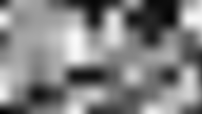
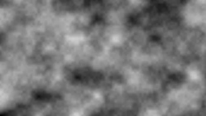
What is needed is a structured form of randomness, where nearby points in space produce similar values. This is the principle behind value noise: a grid of pseudo-random values is defined in space, and smooth interpolation is applied between them. The result appears random but exhibits greater continuity. A comparison of white noise and value noise with their respective cloud renders is shown in Figure 24.
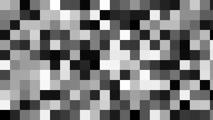
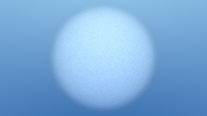
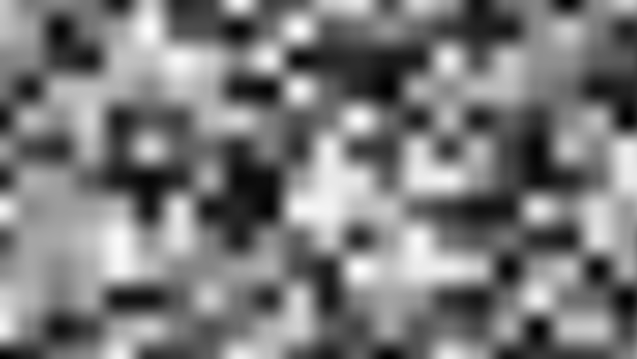
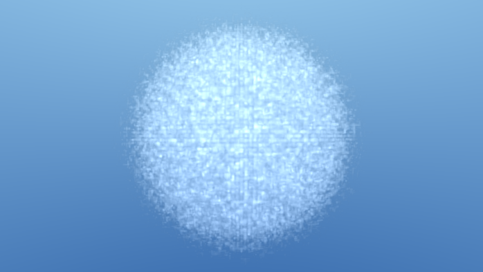
Figure 24 — Comparison of White Noise and Value Noise for cloud generation.
While value noise introduces better variation, it still produces patterns
that lack the complexity of a real cloud. To overcome this limitation,
multiple layers of noise can be combined at different scales in a technique
known as
fractal Brownian motion (fBm) [Musgrave et al.]. For each successive layer (or octave), a higher frequency and lower amplitude are used. By applying fBm within
the getDensity
function, the cloud surface becomes more irregular and visually convincing.
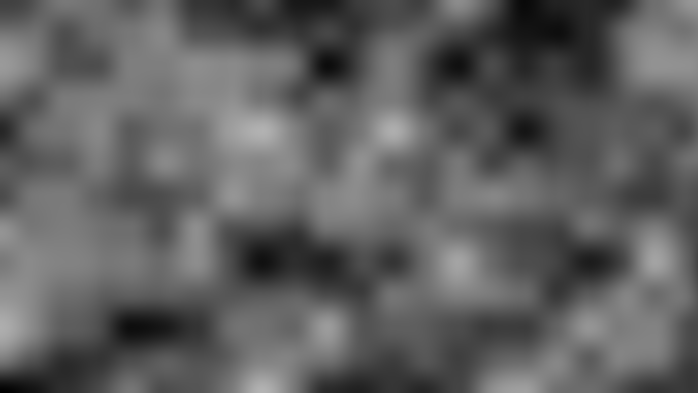
Figure 25 shows the 2D construction of the fBm with each layer and the corresponding cloud render, where the noise is evaluated in three dimensions rather than two.
valueNoise(uv)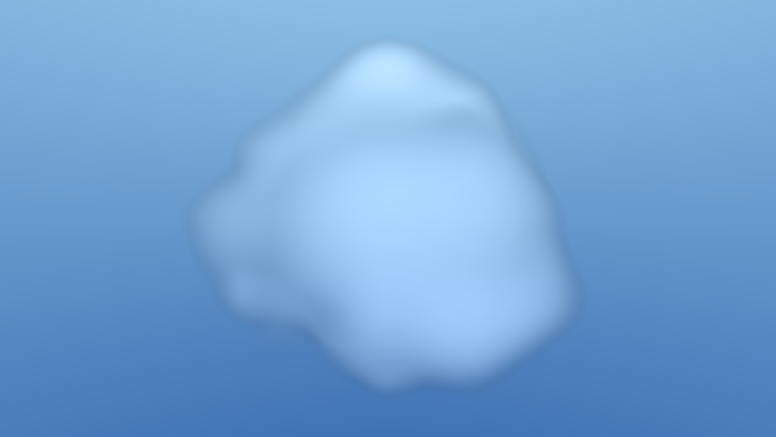
vn(uv)+vn(uv*2.)*0.5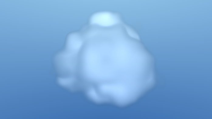

vn(uv)+vn(uv*2.)*0.5+vn(uv*4.)*0.25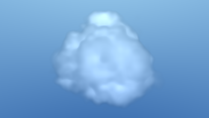
...vn(uv*4.)*0.25+vn(uv*8.)*0.125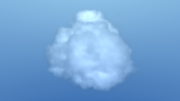
Figure 25 — fBm Noise and Corresponding Cloud Examples with Increasing Octaves.
Volumetric Shading
In the current implementation, cloud rendering does not account for scene illumination. To approximate the interaction between light and the volumetric medium, an efficient technique is employed: at each sampling position, the algorithm advances a short distance along the direction of the incoming light and evaluates the density at this secondary location.
- When the density is higher at the second position, the medium is locally thicker, resulting in increased light scattering.
- When the density decreases, the cloud is less dense, leading to reduced scattering.
vec3 ldir = -normalize(light.direction);
vec3 li = light.color * (light.intensity / (4. * PI));
diffuse = clamp(
    (getDensity(marchPos, scene) - getDensity(marchPos + 0.3 * ldir, scene)) / 0.3,
    0.0, 1.0
);
accumulatedDiffuseColor += mix(vec3(0.), li, diffuse);
Code 11: Lighting the Cloud Volume
Because this technique only compares two nearby points, it is computationally inexpensive yet still captures the essential behavior of light within the volume.
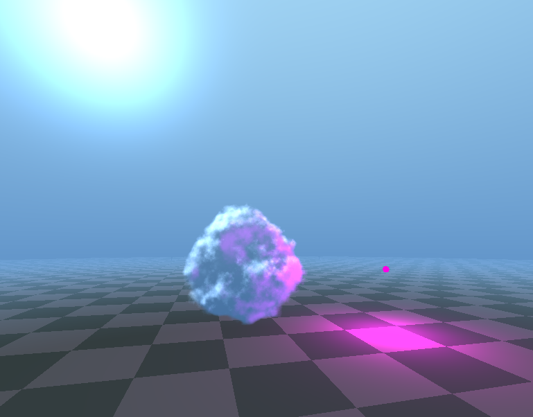
A demonstration of this lighting approximation is shown in Figure 26: a raymarched cloud lit from a white directional light and a pink point light.